

Analysis and selection of models for reservoir inflow simulation in the Ba River Basin
Main Article Content
Abstract
Long-term and accurate daily and monthly streamflow data play a crucial role in understanding hydrological regimes and managing water resources; however, such records are often incomplete, particularly for reservoir inflows. This study addresses this gap by evaluating and comparing the performance of a process-based model (SWAT) and a data-driven model (Light Gradient Boosting Machine – LGBM) in simulating daily and monthly inflows to six major reservoirs in the Ba River Basin, Vietnam – a basin strongly influenced by reservoir regulation for irrigation and hydropower. Observed meteorological, hydrological, and satellite-derived datasets from 2016 to 2023 were utilized, with the period from 2017 to 2022 allocated for calibration and training, and 2016 and 2023 reserved for independent validation. SWAT calibration was performed automatically with SWAT-CUP, while the hyperparameters of LGBM were optimized using Bayesian Optimization (BOA). The results demonstrate the superior performance of LGBM in most cases, achieving higher Nash–Sutcliffe Efficiency (NSE) and Kling–Gupta Efficiency (KGE) scores, and reproducing key hydrological signatures more accurately than SWAT. Nevertheless, SWAT exhibited comparatively better performance in simulating monthly inflows to the An Khe reservoir, highlighting the potential advantages of process-based models under specific conditions.
Keywords
Hydrological modelling, SWAT, Machine learning, LGBM, Reservoir inflow
Article Details

This work is licensed under a Creative Commons Attribution 4.0 International License.
Introduction
In hydrological and water resources studies, long-term daily and monthly streamflow data play a critical role (Khatibi et al., 2012). The most accurate possible time series of streamflow is fundamental for gaining in-depth insights into river flow variability and is essential for assessing the impacts of climate change on streamflow as well as for characterizing the hydrology and water resources of a study area (Gao et al., 2020; Adnan et al., 2020). However, in most river basins, streamflow has only been observed over relatively short periods, particularly for inflow data to reservoirs. The Ba River Basin in Vietnam is a typical case: systematic and continuous records of reservoir inflows have only been available since 2016. Reconstructing historical inflow data before this period is therefore of great importance for analyzing streamflow regimes and assessing changes in reservoir inflows. Accordingly, this study focuses on reconstructing long-term daily and monthly streamflow data for the major reservoirs in the Ba River Basin, Vietnam.
Currently, there are two principal approaches for simulating streamflow time series: the physically based approach and the data-driven approach. In the physically based approach, hydrological and hydraulic models are developed to estimate streamflow based on relevant physical factors, including meteorological and climatic variables (e.g., precipitation, evapotranspiration, temperature) as well as catchment characteristics (e.g., topography, geology, soils, and land cover). Physically based models consist of mathematical equations representing conceptual models and physical laws, such as the conservation of mass and momentum (Chua, 2012). These models have been widely applied to predict various hydrological variables, including streamflow (Ouyang et al., 2021; Kumar et al., 2023). However, handling hydrological parameters in physically based models requires high-quality datasets and detailed knowledge of watershed processes (Woo et al., 2021).
Data-driven models have also been extensively employed to simulate and forecast streamflow in hydrological studies (Evora & Coulibaly, 2009; Elshorbagy et al., 2010; Chang et al., 2015; Yaseen et al., 2016; Ouyang et al., 2021; Khosravi et al., 2021; Hu et al., 2021). These models have become increasingly popular with advances in computational techniques and capabilities over recent decades. Unlike physically based models, data-driven models can be trained relatively easily without requiring in-depth knowledge of physical watershed processes, making them particularly useful in catchments with complex terrain or limited data availability (Wunsch et al., 2018). They can be developed rapidly with minimal input requirements (Asl-Rousta et al., 2018). However, data-driven models are often limited in their ability to provide explicit interpretability of results (Elshorbagy et al., 2010). For instance, some data-driven methods - such as machine learning models and deep learning models-adopt a “black-box” approach, since they mainly rely on data-driven input-output mappings rather than explicit physical representations (Kanungo et al., 2006).
Todini (2007) emphasized the need for comparative assessments of the uncertainty and strengths of physically based versus data-driven models. However, studies that directly compare these two approaches remain limited. Several works (Demirel et al., 2009; Jimeno-Sáez et al., 2018; Ahmadi et al., 2019; Pradhan et al., 2020; Rabezanahary Tanteliniaina et al., 2021; Woo et al., 2021) have compared the Soil and Water Assessment Tool (SWAT) with various machine learning (ML) models in streamflow prediction. These studies generally conclude that data-driven models outperform their physically based counterparts. Nevertheless, such comparisons are usually conducted in catchments that are nearly natural and benefit from high-quality datasets. Evaluating model performance in catchments where hydrological processes are heavily influenced by agricultural activities and artificial reservoirs remains far more challenging (Özdoğan-Sarıkoç & Dadaser-Celik, 2024).
In this study, we aim to contribute to this research gap by applying a physically based model, SWAT (Srinivasan et al., 1998), and a data-driven model, LGBM, to simulate both daily and monthly streamflow in a data-scarce catchment strongly regulated by reservoirs.
The SWAT is a semi-distributed, physically based hydrological model operating at a daily time step (Arnold & Allen, 1996). Its semi-distributed structure enables the simulation of hydrology, sediment, and nutrient dynamics to evaluate watershed behavior (Srinivasan et al., 1998). SWAT is among the most widely used physically based models to characterize basin-scale hydrological processes and to simulate streamflow, reservoir storage, and reservoir operations (Kim & Parajuli, 2012). Numerous applications of SWAT to daily and monthly streamflow simulations (Arnold et al., 1998; Liu et al., 2006; Luo et al., 2012; Yang et al., 2014; Ikenberry et al., 2017) have demonstrated results ranging from satisfactory to good, highlighting the model’s potential for streamflow simulation and justifying its selection in this study.
LGBM, developed by Microsoft in 2016, is a high-performance machine learning algorithm known for its speed, distributed learning capability, open-source availability, and superior gradient boosting performance. LGBM has been successfully applied in hydrological modeling: Yu & Yang (2024) employed LGBM alongside other ML and deep learning models for monthly streamflow simulation in the Pearl River Basin, China, benchmarking against the rainfall-runoff model WAPABA. Similarly, Tran et al. (2025) used LGBM to reconstruct streamflow at the Po Lech station in the Da River Basin, comparing its performance with the VIC hydrological model. Bian et al. (2023) applied LGBM, LSTM, and a hybrid LSTM-LGBM framework to enhance streamflow simulation accuracy in the Shiyang River Basin, while Meyer (2024) used LGBM to simulate streamflow in a Swiss catchment, comparing it with the conceptual PREVAH model. Across these studies, LGBM consistently achieved strong performance, with computational speed being a key advantage over other ML algorithms and physically based models. These strengths underpin its selection for the present study.
This research focuses on the Ba River Basin in Vietnam, a catchment characterized by numerous reservoirs that profoundly regulate streamflow. Hydrological modeling in such a setting is complicated by uncertainties associated with water use for irrigation and hydropower operations, as well as limitations in input datasets such as land use/cover and soil properties. The objective of this study is to evaluate and compare the capabilities of a physically based model (SWAT) and a data-driven model (LGBM) in simulating daily and monthly inflows to major reservoirs in the Ba River Basin. The analysis not only highlights the strengths and limitations of these two modeling approaches but also provides insights into their potential applications for streamflow simulation in the Ba River Basin and similarly challenging catchments worldwide.
Materials and Methods
Research materials
a) Study area
The Ba River Basin is one of the largest river basins in Vietnam and the largest in the South Central region, spanning three provinces: Gia Lai, Dak Lak, and Quang Ngai, with a total catchment area of 14,113 km² (including the Ban Thach tributary). Originating from Mount Ngoc Ro (1,549 m) of the Truong Son Mountain Range, the basin is shaped like an inverted “L,” characterized by narrow upstream and downstream sections, while the middle reaches broaden and receive inflows from 36 first-order and 54 second-order tributaries. Among these, the three main first-order tributaries are the Ayun River (2,950 km²), the Krong H’nang River (1,840 km²), and the Hinh River (1,040 km²), all located on the right bank of the Ba River.
The basin is heavily regulated by a dense cascade of multipurpose reservoirs for irrigation and hydropower, fragmenting the main river into a series of short river-lake segments. Some major reservoirs in the basin include Kanak, An Khe, Ayun Ha, Krong H’nang, Song Ba Ha, and Song Hinh (see Fig. 1). To investigate streamflow dynamics under reservoir regulation, this study focuses on assessing the performance of streamflow simulations at these key reservoirs.
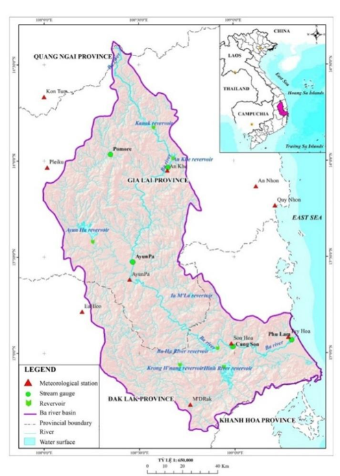
Figure 1. The study area - Ba River Basin, Vietnam
b) Used data
The datasets employed in this study comprise both ground-based observations and remotely sensed data. The locations of ground-based monitoring stations are shown in Fig. 1. Ground observations include water level and discharge records at three hydrological stations: An Khe, Pomore, and Cung Son (source: Vietnam Meteorological and Hydrological Administration); rainfall, evaporation, humidity, sunshine hours, and wind speed from three meteorological stations: An Khe, Buon Ho, and M’Drak; and inflow data for the Kanak, An Khe, Krong H’nang, Song Hinh, and Song Ba Ha reservoirs (source: Ministry of Industry and Trade). Both the SWAT and LGBM models were provided with equivalent hydrometeorological input information to ensure methodological consistency. No additional reservoir operation rules or upstream inflow information were incorporated exclusively into either model.
Satellite data consists of precipitation estimates from the CHIRPS dataset (Funk et al., 2015), aggregated as averages for each sub-basin corresponding to hydrological control points. All datasets were consistently collected for the period 2016-2023. For model development, data from 2017 to 2022 (2191 sample) were used for calibration/training, while data in 2016 and 2023 (731 sample) were reserved for independent validation. In addition, the SWAT model requires a comprehensive set of spatial inputs, including topography, soil, land use, and vegetation cover. The digital elevation model (DEM) used in this study is the void-filled, 1 Arc-second (30 m) product derived from the Shuttle Radar Topography Mission (SRTM) (Doshi, 2014). The soil data were obtained from the Food and Agriculture Organization (FAO) Digital Soil Map of the World, Version 3.5 (Food and Agriculture Organization of the United Nations, 1995) (Fig. 2).
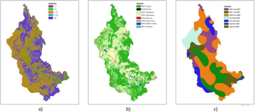
Figure 2. Map of slope (a), land cover (b), and soil (c) in the Ba River Basin
Research methodology
Methodological framework
Figure 3 outlines the overall research methodology. A consistent pre-processing procedure, comprising outlier handling and gap-filling, was applied to the raw input data to ensure data integrity and enhance model performance.
The configuration of the physically-based SWAT model followed a sequential process: (1) generating flow direction and accumulation grids, (2) reclassifying and overlaying spatial layers, (3) delineating the watershed and subbasins, (4) defining land use-soil-slope combinations, and (5) establishing Hydrologic Response Units (HRUs). Subsequent calibration was performed automatically using the SWAT-CUP tool.
For the data-driven LGBM model, data preparation consisted of three key steps. First, input feature selection was performed using the Correlation-based Feature Selection (CFS) algorithm, applied exclusively to the training dataset to identify predictors strongly related to the target variable (Doshi, 2014). Second, feature scaling was conducted using a Min-Max Scaler, where scaling parameters were derived from the training data and subsequently applied to the testing data to prevent data leakage (Deepa & Ramesh, 2022). Third, a chronological split was adopted, with data from 2017-2022 used for training and data from 2016 and 2023 reserved for independent testing to evaluate model generalization across both earlier and later hydrological conditions. Hyperparameter optimization was conducted within the training period using a Bayesian Optimization Algorithm (BOA) (Tran et al., 2025), which performed 100 iterations over a predefined search space. The testing data were not involved in the tuning process, ensuring an unbiased evaluation of model performance.
Model performance was rigorously assessed using a suite of quantitative metrics - including Root Mean Square Error (RMSE), NSE, Mean Absolute Error (MAE), and KGE (Moriasi et al., 2015; Adnan et al., 2017; Liu et al., 2022; Chen et al., 2023) - complemented by an analysis of key hydrological signatures (Westerberg & McMillan, 2015; McMillan, 2021). Comprehensive details for each method are elaborated in Sections 2.3 to 2.6.
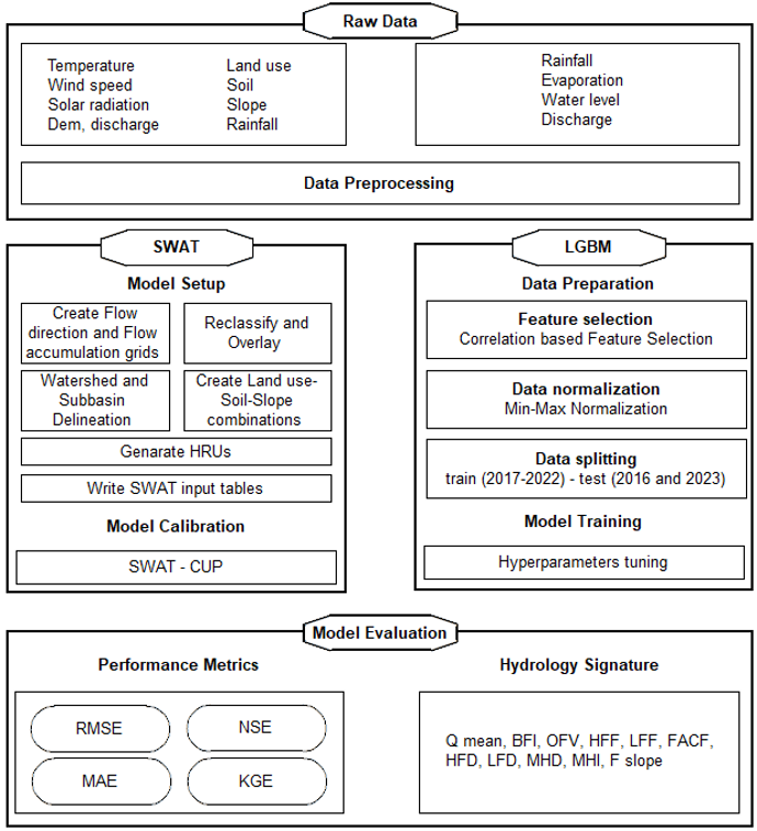
Figure 3. Flowchart of the proposed methodological framework
Physical based model - SWAT model development
a) Model setup
The SWAT is a physically based, semi-distributed hydrological model designed to simulate the impact of land management practices on water, sediment, and agricultural chemical yields in large, complex watersheds over long periods of time (Srinivasan et al., 1998). SWAT divides the watershed into multiple sub-basins, which are further discretized into Hydrological Response Units (HRUs) based on unique combinations of land use, soil type, and slope. This structure allows the model to capture spatial heterogeneity of watershed characteristics while maintaining computational efficiency. The soil water balance is conceptualized in SWAT using Equation (1):
(1)
in which i is the time, SWt is the final soil water content at day i (mm H2O); SWo is the initial soil water content, P is precipitation value, Qsurf is surface runoff value, Ea is the actual evapotranspiration value, wseep is the percolation entering the vadose zone from the soil profile, and Qgw is the value of streamflow originating from groundwater, all measured in mm H2O on day i. The reference evapotranspiration (ET0) is computed with meteorological input data (Neitsch et al., 2005).
For the Ba River Basin, the model setup followed standard SWAT procedures: (1) watershed and sub-basin delineation from the Digital Elevation Model (DEM), (2) overlay of land use, soil, and slope layers to define HRUs, (3) input of daily climate forcing data (precipitation, temperature, wind speed, relative humidity, and solar radiation), and (4) specification of reservoir data and information to account for the significant regulation by multiple dams in the system (daily inflow, outflow, and information regarding reservoir water level, area, and storage according to different operational level). The Ba basin was divided into 75 sub-basins and 1051 HRUs.
b) Parameter- sensitivity analysis, model calibration
Sensitivity analysis and calibration are essential steps to ensure that the SWAT model adequately reproduces hydrological processes in the Ba River BasinBasin. Sensitivity analysis identifies the most influential parameters affecting streamflow simulations (Table 1), which helps reduce model dimensionality and focus calibration efforts on key processes (van Griensven et al., 2006). Parameters commonly reported as sensitive in SWAT studies include the curve number (CN2), soil available water capacity (SOL_AWC), baseflow alpha factor (ALPHA_BF), groundwater delay (GW_DELAY), effective hydraulic conductivity in channel (CH_K2), and threshold water depth in shallow aquifer for return flow (GWQMN) (Arnold et al., 2012). These parameters represent critical components of surface runoff, groundwater contributions, and channel flow dynamics.
In this study, sensitivity analysis was carried out using the SUFI-2 algorithm within SWAT-CUP which applies Latin hypercube sampling to systematically vary parameter ranges and evaluate the corresponding uncertainty in model outputs (Abbaspour et al., 2007). The global sensitivity was quantified through t-stat and p-value measures, where a larger absolute t-statistic and smaller p-value indicate higher sensitivity of the parameter. The most sensitive parameters identified were then prioritized for calibration. The calibration process involved iterative adjustment of sensitive parameters within physically meaningful ranges until an optimal balance was achieved between observed and simulated streamflow at reservoir inflow stations. The objective functions included conventional statistical performance indices e.g. NSE, KGE, RMSE, which are widely recognized as robust measures of hydrological model performance (Moriasi et al., 2015).
Table 1. Selected parameters for sensitivity analysis and calibration/validation
Parameter | Description |
CN2.mgt | Curve number |
ALPHA_BF.gw | Baseflow alpha factor |
GW_DELAY.gw | Groundwater delay time |
GWQMN.gw | Threshold depth of water in the shallow aquifer for return flow to occur |
CH_N2.rte | Manning's "n" value for the main channel. |
CH_K2.rte | Effective hydraulic conductivity in main channel alluvium |
SURLAG.bsn | Surface runoff delay time |
ESCO.hru | Soil evaporation compensation factor |
SOL_K.sol | Saturated hydraulic conductivity (topsoil layer) |
SOL_AWC.sol | Available water capacity (topsoil layer) |
REVAPMN.gw | Threshold depth of water in the shallow aquifer for “revap” to occur |
OV_N.hru | Manning's "n" value for overland flow |
RCHRG_DP.gw | Deep aquifer percolation fraction |
Data based model (LGBM) development
LGBM belongs to the Gradient Boosting Decision Tree (GBDT) family. It stands out due to two innovative techniques: Gradient-based One-Side Sampling (GOSS) and Exclusive Feature Bundling (EFB), which allow it to efficiently handle large datasets and high-dimensional feature spaces. In the GOSS method, training instances are ranked in descending order based on the absolute value of their gradients. Then, 'A'- a subset of the illustrations is attained by keeping the top-a * 100% instance with higher gradients. Then, the remaining set with (1- a) * 100% instances is further randomly sampled to a subset B of size b * . Finally, the consistent objects are split at vector with the estimated variance gain over the subsets A and B, and is given by Equation 2.
(2)
where estimated variance gain over the subset A∪B, = {: }, = {∈ A: > d}, = {∈ B: }, = {∈ B:> d}, and the coefficient is used to normalize the sum of the gradients over B back to the size of . Thus, the estimated is used over a smaller instance subset, instead of the accurate over all the instances to determine the split point. Specifically, j denotes the feature index, and d represents the candidate split threshold for feature j in the decision tree. The subsets A and B correspond to the instances with large gradients and the randomly sampled instances with small gradients, respectively. The subscripts l and r indicate the left and right child nodes after splitting at threshold d. The coefficient (1−a)/b is used to re-weight the gradients of subset B to approximate the contribution of the full dataset. At the same time, the EFB technique is used by LightGBM to minimize the model complexity by bundling the exclusive features into a single feature (Ke et al., 2017).
The LightGBM model in this study was implemented using the lightgbm library for Python (v. 3.10.11). To automate hyperparameter tuning, we employed a Bayesian Optimization algorithm via the bayesOpt library's BayesianOptimizationclass. The optimization process was run for 100 iterations, guided by the Negative Mean Squared Error (-MSE) as the loss function. Maximizing this metric is directly equivalent to minimizing the model's mean squared error.
Input feature selection was using the CFS algorithm (Doshi, 2014) to identify the most relevant predictors for the target variable. A custom Python script calculated the CFS Merit Index for feature subsets. The Merit Index evaluates feature subsets based on two criteria: 1) their collective predictive power (high correlation with the target), and 2) their lack of redundancy (low correlation with each other), ensuring the final selected set contains only the most informative and non-redundant predictors.
Performance metrics
The use of evaluation metrics is a crucial aspect of assessing and comparing the performance of machine learning models. In this study, the selected evaluation metrics include KGE, NSE, MAE, and RMSE. These metrics are considered standard for evaluating the performance of hydrological models, as they measure the discrepancy between the model's simulated or simulated values and observed real-world data (Moriasi et al., 2015; Adnan et al., 2017; Liu et al., 2022; Chen et al., 2023), as detailed below:
- RMSE measures the average error of the model compared to actual data. It is calculated as the square root of the mean of the squared differences between simulated and observed values. A lower RMSE indicates a better-performing model.
(3)
- NSE measures model performance by comparing the sum of squared differences between observed
and simulated values with the sum of squared differences between observed values and their mean. An NSE value closer to 1 indicates a more accurate model.
(4)
- MAE represents the sample mean of the absolute differences between simulated and actual values, where all deviations are weighted equally. A lower MAE indicates a better-performing model.
(5)
- KGE simultaneously integrates bias, variability, and correlation between simulated and observed values. A KGE value closer to 1 indicates a more accurate model:
(6)
Where: represent the ith simulated and observed values, respectively; and denote the mean values of the forecasts and observations; and , are the standard deviations of the simulated and observed values, respectively.
Hydrological signatures
Common performance metrics such as the MSE, NSE, MAE, and KGE are widely used to assess the overall trend and the general agreement between model predictions and observed data. However, these aggregate measures often fail to capture critical hydrological characteristics. Therefore, the principal objective of hydrological modeling shifts to accurately reproducing essential hydrological signatures, which are vital for informing water resource management strategies and conserving the natural processes that sustain aquatic ecosystems (Tran et al., 2025).
Table 2. Hydrology Signatures
Signature | Name | Description | Unit |
Qmean | Mean Flow | Mean flow for the analysis period (2016-2023) | m3/s |
BFI | Base-flow index | Contribution of base flow to total streamflow | - |
OFV | Overall flow variability | Coefficient of variation in streamflow, - i.e. standard deviation divided by mean flow | - |
HFF | High-flow event frequency | Average number of daily high-flow events per year, with a threshold of 9 times the median daily flow | yr-1 |
LFF | Low-flow event frequency | Average number of daily low-flow events per year, with a threshold of 0.2 times the mean daily flow | yr-1 |
HFD | High-flow event duration | Average duration of daily flow events higher than 9 times the median daily flow | days |
LFD | Low-flow event duration | Average number of daily low-flow events per year, with a threshold of 0.2 times the mean daily flow | days |
MHD | Mean half-flow date | The average time of year when the total cumulative flow reaches half the total annual flow | days |
MHI | Mean half-flow interval | The period between the day when half of the total flow of the flood season is reached and the day when half of the total flow of the dry season is reached. | days |
Fslop | Slope of the FDC | Slope of the FDC between the 33 and 66% - exceedance values of streamflow, normalised by its mean | - |
FACF | Flow Auto-Correlation Function | Quantifies how today's flow is statistically related to the flow from previous days | - |
For daily streamflow simulation, this study moves beyond standard performance metrics by employing a suite of 11 hydrological signatures, developed by Westerberg and McMillan (2015) and McMillan (2021), to conduct a more comprehensive model evaluation. The names and detailed descriptions of these signatures are provided in Table 2. These indices are designed to quantitatively capture key aspects of the daily flow regime, including the intensity, frequency, and duration of hydrological events, as well as flow variability and response dynamics. By reflecting core physical watershed processes - such as water transport, storage, and release - these signatures provide a more profound assessment than conventional error metrics alone. This evaluation approach not only tests the statistical accuracy of the simulated hydrograph but also validates the model’s capacity to accurately represent the integrated hydrological behaviour of the watershed, thereby offering a holistic perspective on the strengths and limitations of each modelling approach.
Results
Results of daily flow simulation
Figure 4 presents the daily streamflow series from 2016 to 2023 at the six study sites, alongside the corresponding simulations generated by the SWAT and LGBM models. The period from 2017 to 2022 was used for model calibration/training, while the data in 2016 and 2023 were reserved for model validation.
Overall, the LGBM model demonstrated a superior capacity for learning and achieved higher performance in simulating daily streamflow, with its estimates aligning more closely with the observed data than those of the SWAT model. However, both models struggled to accurately capture peak flood flows at the two upstream reservoirs, Ka Nak and An Khe. Notably, at Ka Nak, the SWAT model exhibited a phase-shift phenomenon. Furthermore, simulated results from both models displayed a consistent tendency to overestimate flow during the dry season.
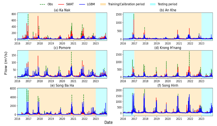
Figure 4. Observed and Simulated Daily Streamflow of SWAT and LGBM model
At the remaining four sites, the LGBM model proved to be markedly superior, as its simulated hydrographs consistently adhered more closely to the observations than those of SWAT. This was particularly evident at the Song Hinh reservoir, where the discrepancy in peak flood values was minimal.
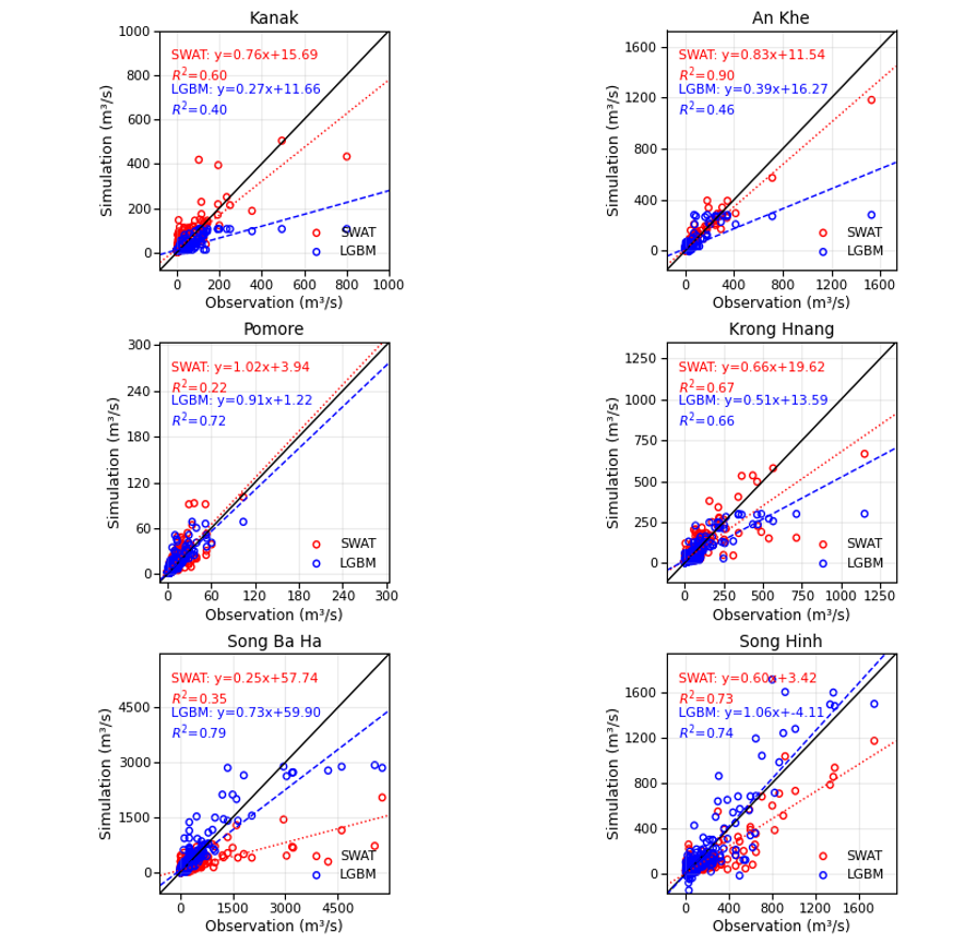
Figure 5. Scatter plot of model’s performance for simulating daily flow
Figure 5 presents a scatter plot of simulated values from the SWAT and LGBM models against the corresponding observed streamflow data. The plot clearly indicates that the SWAT model simulations exhibit greater deviation from the observed values compared with those of the LGBM model. This discrepancy is particularly pronounced at the Ka Nak reservoir and the Pomore hydrological station. For low-flow conditions (dry season periods), the LGBM model generally performed well, demonstrating a good ability to simulate baseflow. However, during high-flow events, particularly for extreme flood peaks, the LGBM model encountered significant difficulties. It consistently underestimated these peak values, failing to capture their magnitude accurately. This systematic underestimation of high flows is notably evident at the Song Ba Ha reservoir and the Krong H’nang station.
Table 3. Results of the Daily Streamflow Simulation Models (testing period)
Computational Point |
| Performance metrics | ||||||||
SWAT |
| LGBM | ||||||||
RMSE | NSE | MAE | KGE |
| RMSE | NSE | MAE | KGE | ||
Ka Nak | 27.98 | 0.54 | 14.84 | 0.49 |
| 35.75 | 0.52 | 16.88 | 0.62 | |
An Khe | 19.64 | 0.86 | 11.10 | 0.78 |
| 37.43 | 0.55 | 12.80 | 0.50 | |
Pomore | 7.09 | 0.43 | 4.93 | 0.46 |
| 4.09 | 0.81 | 1.75 | 0.87 | |
Krong H’nang | 49.35 | 0.59 | 21.24 | 0.59 |
| 48.20 | 0.60 | 14.62 | 0.54 | |
Song Ba Ha | 313.2 | 0.35 | 127.02 | 0.17 |
| 142.23 | 0.87 | 47.26 | 0.87 | |
Song Hinh | 86.11 | 0.65 | 41.4 | 0.51 |
| 53.35 | 0.87 | 25.63 | 0.93 | |
Table 3 presents the performance metrics for the daily streamflow simulations over the entire period from 2016 to 2023 (testing results only; training results are provided in Table S1 in the Supplementary Information). Overall, the LGBM model outperformed the SWAT model across all evaluated indices. The SWAT model demonstrated limited effectiveness, with NSE values below the minimum satisfactory threshold of 0.5 at some study sites, particularly at the Pomore hydrological station and the Song Ba Ha reservoir, where NSE values reached only 0.43 and 0.35, respectively.
At the An Khe and Ka Nak reservoir, the LGBM model also struggled to achieve satisfactory performance, with both its NSE and KGE values ranging only from 0.5 to approximately 0.6. In contrast, the LGBM model exhibited excellent performance at the Song Ba Ha reservoir, Song Hinh reservoir, and the Pomore station, where both NSE and KGE exceeded 0.8. At the Krong H’nang and An Khe reservoirs, the model’s performance was marginally acceptable, just meeting the minimum required thresholds.
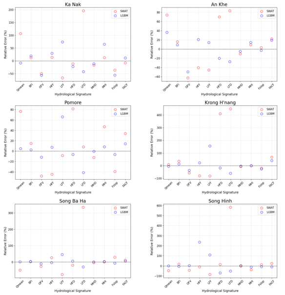
Figure 6. Percentage deviation of hydrological signatures between simulated and observed data
The evaluation of percentage errors (%) relative to observed data for 11 hydrological signatures across six study sites during the 2016-2023 period (see Fig. 6) reveals a clear distinction in simulation performance between the SWAT and LGBM models. Overall, the LGBM model demonstrated superior accuracy, with significantly lower percentage errors for most metrics compared to the SWAT model. The advantage of the LGBM model was particularly evident in signatures related to water volume, such as mean flow (Qmean), baseflow ratio, overall flow variability (OFV), and flow correlation coefficient.
At the upstream sites - An Khe, Ka Nak, and Pomore - the error values of both models differed substantially across most signatures. The three metrics with the largest discrepancies were Qmean, high-flow duration (HFD), and low-flow duration (LFD). In contrast, at the Song Ba Ha, Song Hinh, and Krong H’nang reservoirs, the LGBM model more accurately simulated both the magnitude and timing of flow variations, demonstrating its higher precision in daily streamflow modeling compared to the SWAT model.
Results of monthly flow simulation
Figure 7 displays the monthly streamflow series from 2016 to 2023 at the six study sites. In general, the rapid rise of flood flows at the reservoirs posed challenges for both the SWAT and LGBM models, particularly during the 2016 flood season.
For the SWAT model, simulations at the An Khe reservoir yielded better results than those of the LGBM model. However, at the remaining sites - Ka Nak, Pomore, Song Hinh, and Song Ba Ha - the LGBM model demonstrated a superior ability to capture peak flows as well as subtle fluctuations during dry months. Only the Krong H’nang reservoir exhibited similar performance between the two models.
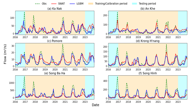
Figure 7. Observed and Simulated Monthly Streamflow of SWAT and LGBM model
During the calibration/training period, both models simulated flow variations relatively closely to observations. In the validation period, however, the data-driven LGBM model maintained higher accuracy. Specifically, at the Ka Nak reservoir, although both models tended to underestimate flows, the LGBM model more effectively simulated flood events in 2016, 2017, 2020, and 2023. Notably, during the validation years (2016 and 2023), SWAT simulations showed significant deviations: a misalignment in the timing of the peak flood month in 2016 and an overestimation in 2023.
Despite being located directly downstream of Ka Nak, results at the An Khe reservoir showed the opposite trend. The SWAT model performed well, capturing flood peaks more accurately than LGBM in most high-flow years (2016, 2017, 2020, 2021, 2022). The LGBM model appeared less capable of reproducing the timing and magnitude of these flood peaks.
At the Krong Hnang reservoir, although the LGBM model achieved better results during the validation period, overall performance throughout the entire simulation period was relatively similar between the two models. The LGBM model more accurately simulated dry-season low flows, while SWAT better captured peak flows during the flood season.
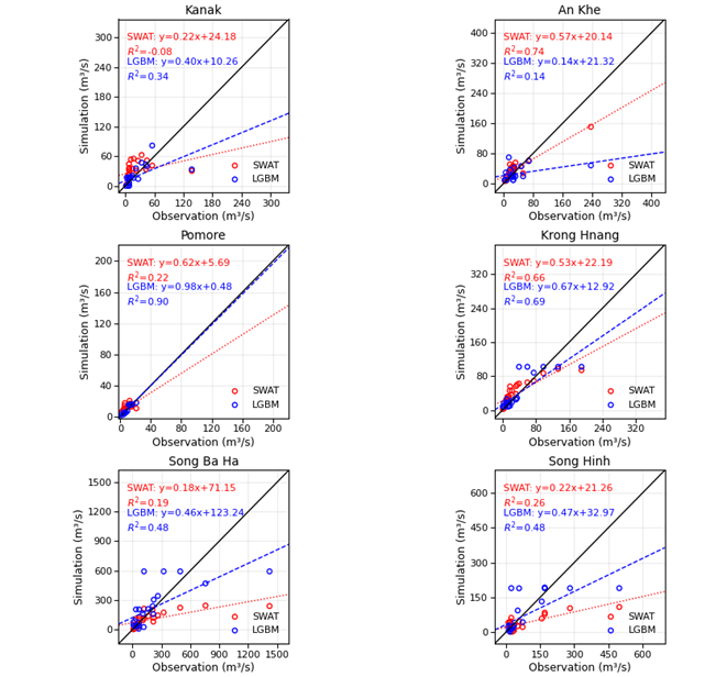
Figure 8. Scatter plot of model’s performance for simulating monthly flow
Figure 8 presents scatter plots comparing the monthly streamflow simulations from the SWAT and LGBM models against observed data. Overall, the LGBM model demonstrated greater stability and closer alignment with observations at low-flow values compared to SWAT.
At the Ka Nak and Krong Hnang reservoirs, SWAT simulations exhibited a tendency to overestimate flows, while the LGBM model showed better agreement with observed values. For peak flood flows, both models tended to underestimate the observations, though the magnitude of underestimation was smaller for LGBM.
At the An Khe and Ba Ha sites, the simulation results showed significant scatter, reflecting the complex influence of reservoir regulation, which posed challenges for both models in accurately replicating the data. In contrast, at the Pomore and Song Hinh sites, the simulated points were more tightly clustered along the perfect-fit line, indicating that the LGBM model performed considerably well in reproducing streamflow. This was particularly evident at Song Hinh, where errors in both average and flood flow simulations were smaller than those of the SWAT model.
Table 4. Results of the Monthly Streamflow Simulation Models (testing period)
Computational Point |
| Performance metrics | ||||||||
SWAT |
| LGBM | ||||||||
RMSE | NSE | MAE | KGE |
| RMSE | NSE | MAE | KGE | ||
Ka Nak | 13.72 | 0.69 | 11.511 | 0.47 |
| 12.77 | 0.71 | 9.74 | 0.65 | |
An Khe | 15.82 | 0.82 | 9.47 | 0.83 |
| 30.91 | 0.30 | 17.28 | 0.29 | |
Pomore | 4.57 | 0.49 | 3.66 | 0.54 |
| 2.33 | 0.87 | 1.53 | 0.87 | |
Krong H’nang | 15.75 | 0.86 | 12.32 | 0.75 |
| 22.11 | 0.83 | 12.14 | 0.78 | |
Song Ba Ha | 210.02 | 0.30 | 113.55 | 0.13 |
| 134.70 | 0.71 | 69.59 | 0.73 | |
Song Hinh | 56.24 | 0.64 | 35.46 | 0.44 |
| 57.98 | 0.69 | 31.21 | 0.68 | |
Table 4 presents the performance metrics for monthly streamflow simulations over the entire period from 2016 to 2023 (testing results only; training results are provided in Table S2 in the Supplementary Information). These evaluation results are fully consistent with the observations from Figure 5, as the LGBM model outperformed SWAT at four of the six study sites: Ka Nak, Pomore, Song Ba Ha, and Song Hinh. The LGBM model achieved Nash-Sutcliffe Efficiency (NSE) values of 0.71, 0.87, 0.71, and 0.69, respectively, compared to SWAT's results of 0.69, 0.49, 0.30, and 0.64.
In contrast, at the An Khe reservoir, the LGBM model performed poorly, with NSE and KGE values of only 0.30 and 0.29, respectively. Meanwhile, the SWAT model demonstrated clear superiority at this site, achieving NSE and KGE values of 0.82 and 0.83.
At the Krong H’nang reservoir, the performance of the two models was comparable. The SWAT model performed better in terms of RMSE and NSE, while the LGBM model achieved superior results for MAE and KGE. However, neither model demonstrated a definitive overall advantage over the other.
Discussion
This study compared the performance of a physically-based model (SWAT) and a data-driven model (LightGBM, or LGBM) for simulating daily and monthly streamflow to reservoirs in the Ba River Basin. Our findings align with a growing body of research demonstrating the efficacy of data-driven approaches in hydrological modeling. For instance, Özdoğan-Sarıkoç and Dadaser-Celik (2024) reported that a NARX model outperformed SWAT in predicting streamflow and reservoir storage, while Tran et al. (2025) found machine learning models superior to the Variable Infiltration Capacity (VIC) model for daily flow simulation.
Consistent with these studies, our results demonstrate the superior performance of the LGBM model. Based on standard performance metrics (NSE, KGE, RMSE, MAE) and its ability to replicate key hydrological signatures (Figure 7), LGBM outperformed SWAT at all six sites for daily flow and at four of the six sites for monthly flow. This underscores the advantage of machine learning models like LGBM in complex, heavily regulated basins where input data for physical models may be limited or uncertain.
The SWAT model produced unsatisfactory results at certain locations, such as Ba Ha and Pomore for daily flow. This poor performance can be attributed to several factors: (1) The high complexity and uncertainty in simulating the operation rules of cascading reservoirs within SWAT. (2) Potential inaccuracies or insufficient detail in input data (e.g., soil parameters, land use, and precise reservoir operation schedules). (3) The inherent difficulty of physical models in capturing rapid, nonlinear hydrological responses in heavily engineered systems. Furthermore, while data-driven models can leverage auxiliary data like stage-discharge relationships (Nguyen et al., 2023) as input features, SWAT does not incorporate such information, potentially putting it at a disadvantage.
A notable exception was observed at the An Khe reservoir for monthly flow, where SWAT performed well and LGBM failed. This anomaly is likely because An Khe is located directly downstream of the Ka Nak reservoir, making its inflow highly dependent on Ka Nak's physical operation rules. SWAT can explicitly represent this physical causality, whereas LGBM may lack the necessary input features to learn this complex, deterministic relationship effectively. This highlights that model superiority is context-dependent; physically-based models remain valuable in systems where dominant processes are well-defined and can be accurately parameterized. Nevertheless, more detailed investigations incorporating explicit reservoir operation data and additional explanatory variables are required to provide a more comprehensive and convincing interpretation of this discrepancy.
Both models exhibited a systematic underestimation of peak flood flows, particularly at upstream reservoirs like Ka Nak. This mutual limitation suggests that neither approach fully captures the extreme flood generation mechanisms in multi-reservoir systems, where emergency operational decisions may not be well-represented in training data or model parameters. Improving the simulation of high-flow events remains a critical challenge for future research.
Finally, the use of hydrological signatures provided deeper insight beyond conventional error metrics. The analysis revealed that LGBM not only achieved numerical accuracy but also more faithfully reproduced the basin's integrated hydrological behavior (e.g., flow frequency, duration, and variability). This comprehensive evaluation strongly reinforces the conclusion of LGBM's overall superiority in this specific basin context.
Numerous studies worldwide have compared data-driven models with the SWAT model (Mirzaei et al., 2021; Jiang et al., 2024; Wang et al., 2025), with most concluding that data-driven models are a viable alternative to the SWAT model. This conclusion is especially true when climate data (temperature and precipitation), physical data (such as soil and land-use maps), and slope data used to define Hydrologic Response Units (HRUs) are inaccurate, inadequate, or influenced by reservoirs (Mirzaei et al., 2021). In their study of the Fenhe River basin, Jiang et al. (2024) noted that although both data-driven and SWAT models proved effective in simulating runoff with notable fluctuations, exploring an approach that combines the two groups should be considered to improve the simulation of peak flow characteristics in the future.
Conclusion
Two primary approaches for simulating river flow processes are physically-based models and data-driven models. Physically-based models utilize established knowledge of hydrological processes to predict the dynamics of a hydrological system. In contrast, data-driven models offer an alternative solution that does not require explicit understanding of the underlying physical processes. For data-driven models, accurately replicating the system's output is prioritized over replicating the specific physical characteristics of the watershed.
This study conducted a comprehensive evaluation of these two distinct modeling approaches for simulating mean daily and mean monthly streamflow to reservoirs within the challenging context of the Ba River Basin - a basin significantly regulated by human activities through irrigation and hydropower operations. Based on an analysis of performance metrics and hydrological signatures, the following key results were obtained:
(1) For daily streamflow simulation, the SWAT model results were just satisfactory at 3 out of 6 study sites. Conversely, the LGBM model results were unsatisfactory only at the Ka Nak reservoir, were average at the An Khe and Krong H'nang reservoirs, and were good at the Pomore station, Song Ba Ha reservoir, and Song Hinh reservoir. Analysis based on hydrological signatures also showed that the simulation results from the LGBM model were relatively good and significantly better than those from the SWAT model.
(2) For monthly streamflow simulation: The LGBM model demonstrated higher performance than the SWAT model at the majority of reservoir sites, effectively reconstructing the monthly flow series with greater accuracy. However, specifically for simulating monthly inflow to the An Khe reservoir, while the LGBM model results were unsatisfactory (NSE and KGE both below 0.5), the SWAT model results were quite good (NSE = 0.82, KGE = 0.83). Therefore, the choice of model should be carefully considered based on the specific objectives and characteristics of each study location.
(3) The SWAT model is a physically-based model that simulates hydrological processes across a watershed. On the other hand, the LGBM model is a data-driven model that does not explicitly account for physical processes. Consequently, comparing these two models is challenging due to their fundamentally different natures. In this study, the LGBM model generally yielded better results than the SWAT model. However, the SWAT model can also perform well in certain scenarios and may be more suitable under changing physical and hydrological conditions, as it better simulates the actual watershed processes.
In summary, this study demonstrates that for the Ba River BasinLGBM modelrepresent a promising and effective tool for reconstructing and simulating long-term streamflow, contributing significantly to enhancing the effectiveness of water resource assessment and management.
Acknowledgments: This research was supported by the project under the code E3.8. Funding was provided by Joint Vietnam-Russia Tropical Science and Technology Research Center.
Data Availability Statement: The data supporting the findings of this study are available from the corresponding author upon reasonable request.
Author Contributions: Dinh Ba Duy, Pozdniakov Shamil, Nguyen Duc Hanh conceived the study and supervised its implementation; Le Huu Minh Quan, Ly Minh Tuan, Nguyen Duc Hanh and Dinh Vu Anh Tu were responsible for data processing; Dinh Ba Duy, Pozdniakov Shamil Raufovich, Pozdniakova Albina Iskandarovna, Shilov Dmitrii Vladimirovich, and Dinh Vu Anh Tu contributed to data analysis, manuscript writing, and editing. All authors read and approved the final version of the manuscript.
Conflict of Interest Statement: The authors declare no financial or other conflicts of interest.
Statement on the Use of Generative AI (GenAI): The authors declare that generative artificial intelligence (GenAI) tools were used only to assist with language editing and improving the clarity of the manuscript. All intellectual content, including the study design, data analysis, interpretation of results, and scientific conclusions, was entirely generated and verified by the authors. The authors carefully reviewed and validated all AI-assisted outputs to ensure accuracy and to avoid the inclusion of incorrect, biased, or fabricated information.
Supplementary Files:
References
Abbaspour, K. C., Vejdani, M., & Haghighat, S. (2007). SWAT-CUP calibration and uncertainty programs for SWAT. In MODSIM 2007 International Congress on Modelling and Simulation (pp. 1603-1609). Christchurch, New Zealand.
Adnan, R. M., Liang, Z., Heddam, S., Zounemat-Kermani, M., Kisi, O., & Li, B. (2020). Least square support vector machine and multivariate adaptive regression splines for streamflow prediction in mountainous basin using hydro-meteorological data as inputs. Journal of Hydrology, 586, 124371. https://doi.org/10.1016/j.jhydrol.2019.124371
Adnan, R. M., Yuan, X., Kisi, O., & Yuan, Y. (2017). Streamflow forecasting of Astore River with seasonal autoregressive integrated moving average model. European Scientific Journal, 13(12), 145-156. https://doi.org/10.19044/esj.2017.v13n12p145
Ahmadi, H., Arji, G., Shahmoradi, L., Safdari, R., Nilashi, M., & Alizadeh, M. (2019). The application of internet of things in healthcare: A systematic literature review and classification. Universal Access in the Information Society, 18(4), 837-869. https://doi.org/10.1007/s10209-018-0618-4
Arnold, J. G., & Allen, P. M. (1996). Estimating hydrologic budgets for three Illinois watersheds. Journal of Hydrology, 176(1-4), 57-77. https://doi.org/10.1016/0022-1694(95)02782-3
Arnold, J. G., Moriasi, D. N., Gassman, P. W., Abbaspour, K. C., White, M. J., Srinivasan, R., Santhi, C., Harmel, D., van Griensven, A., Kannan, N., & Jha, M. K. (2012). SWAT: Model use, calibration, and validation. Transactions of the ASABE, 55(4), 1491-1508. https://doi.org/10.13031/2013.42256
Arnold, J. G., Srinivasan, R., Muttiah, R. S., & Williams, J. R. (1998). Large area hydrologic modeling and assessment part I: Model development. Journal of the American Water Resources Association, 34(1), 73-89.https://doi.org/10.1111/j.1752-1688.1998.tb05961.x
Asl-Rousta, B., Mousavi, S. J., Ehtiat, M., & Ahmadi, M. (2018). SWAT-based hydrological modelling using model selection criteria. Water Resources Management, 32(6), 2181-2197. https://doi.org/10.1007/s11269-018-1925-5
Bian, L., Qin, X., Zhang, C., Guo, P., & Wu, H. (2023). Application, interpretability and prediction of machine learning method combined with LSTM and LightGBM - A case study for runoff simulation in an arid area. Journal of Hydrology, 625, 130091. https://doi.org/10.1016/j.jhydrol.2023.130091
Chang, F. J., Tsai, Y. H., Chen, P. A., Coynel, A., & Vachaud, G. (2015). Modeling water quality in an urban river using hydrological factors-Data driven approaches. Journal of Environmental Management, 151, 87-96. https://doi.org/10.1016/j.jenvman.2014.12.014
Chen, H., Huang, S., Xu, Y.-P., Teegavarapu, R. S. V., Guo, Y., Nie, H., Xie, H., & Zhang, L. (2023). River ecological flow early warning forecasting using baseflow separation and machine learning in the Jiaojiang River Basin, Southeast China. Science of the Total Environment, 882, 163571. https://doi.org/10.1016/j.scitotenv.2023.163571
Chua, L. H. C. (2012). Considerations for data-driven and physically based hydrological models in flow forecasting. IFAC Proceedings Volumes, 45(16), 1025-1030. https://doi.org/10.3182/20120711-3-BE-2027.00036
Deepa, B., & Ramesh, K. (2022). Epileptic seizure detection using deep learning through min max scaler normalization. International Journal of Health Sciences, 6(S1), 10981-10996. https://doi.org/10.53730/ijhs.v6nS1.7801
Demirel, M. C., Venancio, A., & Kahya, E. (2009). Flow forecast by SWAT model and ANN in Pracana basin, Portugal. Advances in Engineering Software, 40(7), 467-473. https://doi.org/10.1016/j.advengsoft.2008.08.002
Doshi, M. (2014). Correlation based feature selection (CFS) technique to predict student performance. International Journal of Computer Networks & Communications, 6(3), 197-204.
Elshorbagy, S., Razavi, S. J., Sauchyn, D., & Wheater, P. H. (2010). Experimental investigation of the predictive capabilities of data driven modeling techniques in hydrology - Part 1: Concepts and methodology. Hydrology and Earth System Sciences, 14(10), 1931-1941. https://doi.org/10.5194/hess-14-1931-2010
Evora, N. D., & Coulibaly, P. (2009). Recent advances in data-driven modeling of remote sensing applications in hydrology. Journal of Hydroinformatics, 11(3-4), 194-201. https://doi.org/10.2166/hydro.2009.036
Food and Agriculture Organization of the United Nations. (1995). The digital soil map of the world and derived soil properties [CD-ROM]. Rome, Italy: Author.
Funk, C., Peterson, P., Landsfeld, M., Pedreros, D., Verdin, J., Shukla, S., Husak, G., Rowland, J., Harrison, L., Hoell, A., & Michaelsen, J. (2015). The climate hazards infrared precipitation with stations -A new environmental record for monitoring extremes. Scientific Data, 2, 150066. https://doi.org/10.1038/sdata.2015.66
Gao, C., Su, B., Krysanova, V., Zha, Q., Chen, C., Luo, G., Zeng, X., Huang, J., Xiong, M., Zhang, L., & Jiang, T. (2020). A 439-year simulated daily discharge dataset (1861–2299) for the upper Yangtze River, China. Earth System Science Data, 12(1), 387-402. https://doi.org/10.5194/essd-12-387-2020
Hu, J., Wu, X., Li, X., & Zhang, Q. (2021). Impacts of land-use conversions on the water cycle in a typical watershed in the southern Chinese Loess Plateau. Journal of Hydrology, 593, 125741. https://doi.org/10.1016/j.jhydrol.2020.125741
Ikenberry, C. D., Soupir, M. L., Helmers, M. J., Crumpton, W. G., Arnold, J. G., & Gassman, P. W. (2017). Simulation of daily flow pathways, tile-drain nitrate concentrations, and soil-nitrogen dynamics using SWAT. Journal of the American Water Resources Association, 53(6), 1251-1266. https://doi.org/10.1111/1752-1688.12569
Jiang, Z., Lu, B., Zhou, Z., & Zhao, Y. (2024). Comparison of process-driven SWAT model and data-driven machine learning techniques in simulating streamflow: A case study in the Fenhe River Basin. Sustainability, 16, 6074. https://doi.org/10.3390/su16146074
Jimeno-Sáez, P., Senent-Aparicio, J., Pérez-Sánchez, J., & Pulido-Velazquez, D. (2018). A comparison of SWAT and ANN models for daily runoff simulation in different climatic zones of peninsular Spain. Water, 10(2), 192. https://doi.org/10.3390/w10020192
Kanungo, D. P., Arora, M. K., Sarkar, S., & Gupta, R. P. (2006). A comparative study of conventional, ANN black box, fuzzy and combined neural and fuzzy weighting procedures for landslide susceptibility zonation in Darjeeling Himalayas. Engineering Geology, 85(3-4), 347-366. https://doi.org/10.1016/j.enggeo.2006.03.004
Ke, G., Meng, Q., Finley, T., Wang, T., Chen, W., Ma, W., Ye, Q., & Liu, T.-Y. (2017). LightGBM: A highly efficient gradient boosting decision tree. Advances in Neural Information Processing Systems, 30, 3146-3154.
Khatibi, R., Sivakumar, B., Ghorbani, M. A., Kisi, O., Kocak, K., & FarsadiZadeh, D. (2012). Investigating chaos in river stage and discharge time series. Journal of Hydrology, 414, 108-117. https://doi.org/10.1016/j.jhydrol.2011.10.026
Khosravi, K., Singh, A., Pradhan, B., Afan, H. A., & Lee, S. (2021). Improving daily stochastic streamflow prediction: Comparison of novel hybrid data-mining algorithms. Hydrological Sciences Journal, 66(9), 1457-1474. https://doi.org/10.1080/02626667.2021.1928673
Kim, H., & Parajuli, P. B. (2012). Impacts of reservoir operation in the SWAT model calibration. In 2012 ASABE Annual International Meeting (p. 1). Dallas, TX, United States.
Kumar, V., Sharma, K. V., Caloiero, T., Mehta, D. J., & Singh, K. (2023). Comprehensive overview of flood modeling approaches: A review of recent advances. Hydrology, 10(7), 141. https://doi.org/10.3390/hydrology10070141
Liu, J., Yuan, X., Zeng, J., Jiao, Y., Li, Y., Zhong, L., & Yao, L. (2022). Ensemble streamflow forecasting over a cascade reservoir catchment with integrated hydrometeorological modeling and machine learning. Hydrology and Earth System Sciences, 26(2), 265-278. https://doi.org/10.5194/hess-26-265-2022
Liu, S., Sun, R., Sun, Z., Li, X., & Liu, C. (2006). Evaluation of three complementary relationship approaches for evapotranspiration over the Yellow River basin. Hydrological Processes, 20(11), 2347-2361. https://doi.org/10.1002/hyp.6048
Luo, Y., Arnold, J., Allen, P., & Chen, X. (2012). Baseflow simulation using SWAT model in an inland river basin in Tianshan Mountains, Northwest China. Hydrology and Earth System Sciences, 16(4), 1259-1267. https://doi.org/10.5194/hess-16-1259-2012
McMillan, H. K. (2021). A review of hydrologic signatures and their applications. Wiley Interdisciplinary Reviews: Water, 8(1), e1499. https://doi.org/10.1002/wat2.1499
Meyer, B. (2024). Performance of different machine learning algorithms in rainfall runoff modelling compared to the conceptual model PREVAH in selected Swiss catchments (Master’s thesis, University of Bern).
Mirzaei, M., Yu, H., Dehghani, A., Galavi, H., Shokri, V., Mohsenzadeh Karimi, S., & Sookhak, M. (2021). A novel stacked long short-term memory approach of deep learning for streamflow simulation. Sustainability, 13, 13384. https://doi.org/10.3390/su132313384
Moriasi, D. N., Gitau, M. W., Pai, N., & Daggupati, P. (2015). Hydrologic and water quality models: Performance measures and evaluation criteria. Transactions of the ASABE, 58(6), 1763-1785. https://doi.org/10.13031/trans.58.10715
Neitsch, S. L., Arnold, J. G., Kiniry, J. R., Williams, J. R., & King, K. W. (2005). Soil and water assessment tool: Theoretical documentation (Version 2005). USDA Agricultural Research Service.
Nguyen, D. H., Nguyen, T. G., Dang, T. D. M., Dao, B. H., Le Huu, M. Q., & Nguyen, T. T. (2023). Modelling stage-discharge relationships for hydrological stations in the Da River Basin using first-kind Chebyshev polynomial approximation. VNU Journal of Science: Earth and Environmental Sciences, 39(2). https://doi.org/10.25073/2588-1094/vnuees.4956
Ouyang, W., Lawson, K., Feng, D., Ye, L., Zhang, C., & Shen, C. (2021). Continental-scale streamflow modeling of basins with reservoirs: Towards a coherent deep-learning-based strategy. Journal of Hydrology, 599, 126455. https://doi.org/10.1016/j.jhydrol.2021.126455
Özdoğan-Sarıkoç, G., & Dadaser-Celik, F. (2024). Physically based vs. data-driven models for streamflow and reservoir volume prediction at a data-scarce semi-arid basin. Environmental Science and Pollution Research, 31(27), 39098-39119. https://doi.org/10.1007/s11356-024-33732-w
Todini, E. (2007). Hydrological catchment modelling: Past, present and future. Hydrology and Earth System Sciences, 11(1), 468-482. https://doi.org/10.5194/hess-11-468-2007
Pradhan, P., Tingsanchali, T., & Shrestha, S. (2020). Evaluation of soil and water assessment tool and artificial neural network models for hydrologic simulation in different climatic regions of Asia. Science of the Total Environment, 701, 134308. https://doi.org/10.1016/j.scitotenv.2019.134308
Rabezanahary Tanteliniaina, M. F., Rahaman, M. H., & Zhai, J. (2021). Assessment of the future impact of climate change on the hydrology of the Mangoky River, Madagascar using ANN and SWAT. Water, 13(9), 1239. https://doi.org/10.3390/w13091239
Rabus, B., Eineder, M., Roth, A., & Bamler, R. (2003). The shuttle radar topography mission-A new class of digital elevation models acquired by spaceborne radar. ISPRS Journal of Photogrammetry and Remote Sensing, 57(4), 241–262. https://doi.org/10.1016/S0924-2716(02)00124-7
Srinivasan, R., Arnold, J. G., & Jones, C. A. (1998). Hydrologic modelling of the United States with the soil and water assessment tool. International Journal of Water Resources Development, 14(3), 315-325. https://doi.org/10.1080/07900629849231
Tran, V. N., Nguyen, H. D., Khuong, H. V., Dao, H. B., Le, Q. H. M., Nguyen, C. Q., & Nguyen, G. T. (2025). Reconstructing long-term daily streamflow data at the discontinuous monitoring station in the ungauged transboundary basin using machine learning. Water Resources Management, 1-22. https://doi.org/10.1007/s11269-025-04109-6
Van Griensven, A., Meixner, T., Grunwald, S., Bishop, T., Diluzio, M., & Srinivasan, R. (2006). A global sensitivity analysis tool for the parameters of multi-variable catchment models. Journal of Hydrology, 324(1-4), 10-23. https://doi.org/10.1016/j.jhydrol.2005.09.008
Wang, J., Yousefi, H., & Shourian, M. (2025). Comparison of process-based hydrological modeling and deep learning approaches for streamflow simulation. Water Resources Management, 39, 7689-7708. https://doi.org/10.1007/s11269-025-04313-4
Westerberg, I. K., & McMillan, H. K. (2015). Uncertainty in hydrological signatures. Hydrology and Earth System Sciences, 19(9), 3951-3968. https://doi.org/10.5194/hess-19-3951-2015
Woo, S. Y., Kim, J. H., Park, J. Y., & Kim, J. (2021). Evaluating the impact of interbasin water transfer on water quality in the recipient river basin with SWAT. Science of the Total Environment, 776, 145984. https://doi.org/10.1016/j.scitotenv.2021.145984
Wunsch, A., Liesch, T., & Broda, S. (2018). Forecasting groundwater levels using nonlinear autoregressive networks with exogenous input (NARX). Journal of Hydrology, 567, 743-758. https://doi.org/10.1016/j.jhydrol.2018.01.045
Yang, F., Zhang, G.-L., Yang, J.-L., Li, D.-C., Zhao, Y.-G., Liu, F., Yang, R.-M., & Yang, F. (2014). Organic matter controls of soil water retention in an alpine grassland and its significance for hydrological processes. Journal of Hydrology, 519, 3086-3093. https://doi.org/10.1016/j.jhydrol.2014.10.054
Yaseen, Z. M., Jaafar, O., Deo, R. C., Kisi, O., Adamowski, J., Quilty, J., & El-Shafie, A. (2016). Stream-flow forecasting using extreme learning machines: A case study in a semi-arid region in Iraq. Journal of Hydrology, 542, 603-614. https://doi.org/10.1016/j.jhydrol.2016.09.035
Yu, H., & Yang, Q. (2024). Applying machine learning methods to improve rainfall–runoff modeling in subtropical river basins. Water, 16(15), 2199. https://doi.org/10.3390/w16152199